Probing the Universe with galaxy clusters

Space is pretty damn big, and from a human perspective, there really is a lot of stuff out there. When we look at something massive like a galaxy cluster, we are inadvertently observing all the objects behind it as well. What we see isn’t an exact representation of where all these background objects actually are on the sky! The massive galaxy cluster bends the path of light as it travels towards us, and in the case of strong lensing, can even create multiple images of the object in question. In this post, I’ll be telling you about how we can use this strong lensing effect to measure relative distances between us, the galaxy cluster and background object, which in turn lets us probe the expansion history of the Universe!

Gravitational lensing and it’s dependence on cosmology

An illustration of strong lensing by a galaxy cluster

We’ll have to start out with a little bit of math to understand how strong lensing can tell us anything about the history of our Universe.

The true angular position of a source galaxy lensed by a galaxy cluster will be given by the lensing equation,

where theta is the observed position, alpha is the deflection angle due to the mass distribution of the lens, and the scaling factor is a ratio between the distance between the source and lens and the distance between the observer and source. This distance is super interesting, since they actually correspond to angular diameter distances!

“What are angular diameter distances?” I hear you ask. These distances are one of the many distances measures we use at cosmological scales, and are defined as the ratio between the physical extent of an object and it’s angular size, as viewed from the Earth. In a Euclidean geometry this simply corresponds to typical distances found using the small angle approximation. Considering our Universe is not Euclidean, however, means that this distance is tightly linked to the geometry of the Universe at large scales.

Returning to the lensing equation, we see that all is not well if we want to measure the geometry of the Universe. The distance factor has a multiplicative degeneracy with the deflection angle, which is found by modelling the mass distribution of the lensing cluster. In the case of more than one multiply lensed source, this degeneracy is reduced and we can get information on the quantity

For N multiply lensed background source we then get N-1 independent distance ratios that give us information on the background cosmology. Hurray!

Expected degeneracy, BayesLens and mock clusters, oh my!

Now that we’ve established the fact that galaxy clusters can, in theory at least, give us information about the background cosmology, we need to determine how degenerate that information is. This is a typical issue for cosmological probes, where multiple different choices of models and parameters lead to the same observable values. Only by combining complementary and independent probes can we break these degeneracies and put constraints on our cosmological models!

We can get an idea of what kind of degeneracies distance ratios will give us by assuming a fiducial cosmology such as LCDM, pairs of source redshifts and lens redshift. We can then calculate the distance ratios we would measure for these lens/source combinations if our fiducial cosmology is correct. An expected degeneracy can then be found by freeing up two (or more) parameters and finding the combinations of parameter values that lead to the same expected distance rations. These kind of plots are important, as they can give us information about what observations we need to make with our telescopes.

Based on earlier literature (to be cited once I figure out squarespace), distance ratios should be most sensitive to the dark energy equation of state parameter, w, and the matter density parameter. The resulting degeneracy can be seen in the Figure below, where I assume a relative error of 5% on the distance ratio measurements.

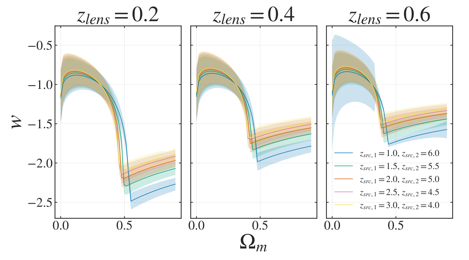
Degeneracy in the w-Omega_m plane for a wCDM cosmology, given different combinations of lens and source redshifts and the corresponding distance rations from a LCDM fiducial cosmology

Now isn’t that beautiful? We see this interesting curvy, L(ish) shape in the degeneracy. We also see that all the curves intersect at the fiducial values of Omega_m = 0.3 and w = -1 (I swear I’ll get LaTex working on here at some point), as we would expect. For all other combinations the lines vary in position, as different cosmologies will be necessary to reproduce the observed distance ratios. This is especially pronounced for high matter densities. What this tells us is that if the observed distance ratios were due to a different cosmology, we would have higher constraining power with multiple lenses/sources for Omega_m < 0.5.

The question now is whether this holds for actual observations. We can test this by simulating galaxy clusters, ray tracing light from background sources to create multiple image families, and then modelling the cluster using some kind of lens model. That’s a woozy of a sentence, hey! The first part, simulation clusters and ray tracing background sources, will be covered in a future blog post. For now, let’s just assume we have some mock clusters at different redshifts (z=[ 0.209, 0.348, 0.439 ]) with a number of lensed images from background sources in the redshift range 1-6.

In my work, I model galaxy clusters using the state-of-the-art BayesLens code. This is a Bayesian hierarchical lensing model that builds on the older LensTool code. Both of these codes model member galaxies as circular dual pseudo-isothermal mass distributions, given by

What this means is not super important, instead one’s attention should be drawn to the number of parameters. If we have on the order of a 100 member galaxies, we suddenly have to model 300 parameters, which might not be feasible. Instead, both codes assume a scaling relation for these 3 parameters that relates them to observed magnitudes for each galaxy. These scaling relations are definied by a set of hyperparameters (The relations will be shown here once LaTeX decides to work for me instead of against me).

Where BayesLens improves upon LensTool is that it determines these hyperparameters based on the observed data, and incorporates a scatter along the relation. In this sense, BayesLens is more “physical” than LensTool, which forces each galaxy to lie on the defined scaling relations.

In my work, I expand on this idea and include the chosen cosmology among the hyperparameters that BayesLens determines based on the data. By doing this, we create a self-consistant piece of modelling software that determines both the lens model and the background cosmology at the same time!

Applying this to the mock clusters mentioned earlier, I get the following result:

Posterior distributions for a wCDM cosmology for a set of 3 mock clusters

And wouldn’t you know it, we see part of this funky L-shape, as mentioned earlier! Huzzah! For illustrative purposes, I’ve also included the Planck18 CMB data, and we see that the lensing measurements are orthogonal-ish to the resulting posterior. The constraining power given by these simulations is still pretty lacking however, and the join distribution is roughly 3-sigma away from the CMB result. This discrepancy is most likely due to the unphysical mock clusters, which only contain 20 member galaxies each. As a proof of concept, however, they function perfectly!

The next step would be to create some realistic mock clusters, with 100s of member galaxies. This, together with a 101 on cluster simulation will be the topic of my next blog post, so stay tuned!